Cell detection and classification
Classify and detect cells in testis histopathology images
Cell detection and classification
Task
Physicians can identify men’s infertility by counting specific cells in testis histopathology images. Such annotation is hard manual labor that can be automated using neural networks. Ida-Tallinn hospital provided a large dataset of these images to build a cell detector and classifier to ease specialists’ lives.
WSI and MIRAX format
Training images WSI (whole slide image) come in MIRAX format - a special kind of virtual slide format. A virtual slide is a high-resolution digital image of the microscopy sample created by sliding the glass past the camera and taking multiple pictures.
These created images are too high-resolution to handle as full images and are broken up into multiple files. This kind of processing needs special notation and a system to view and access data after storage.
On disk the format includes:
.mrxsfile that holds the metadata including information on how.datfiles are organized- data folder with
.datfiles that hold the actual image data Index.datfile in the data folder that holds the pointers to locate the image data.jsonannotation file in JSON format that holds the metadata for the annotated section of the imageSlidedat.inifile in the data folder contains structural data and parameters of the scanning process inkey=valueformat. These values are also used to receive image data.
Example of a single slide
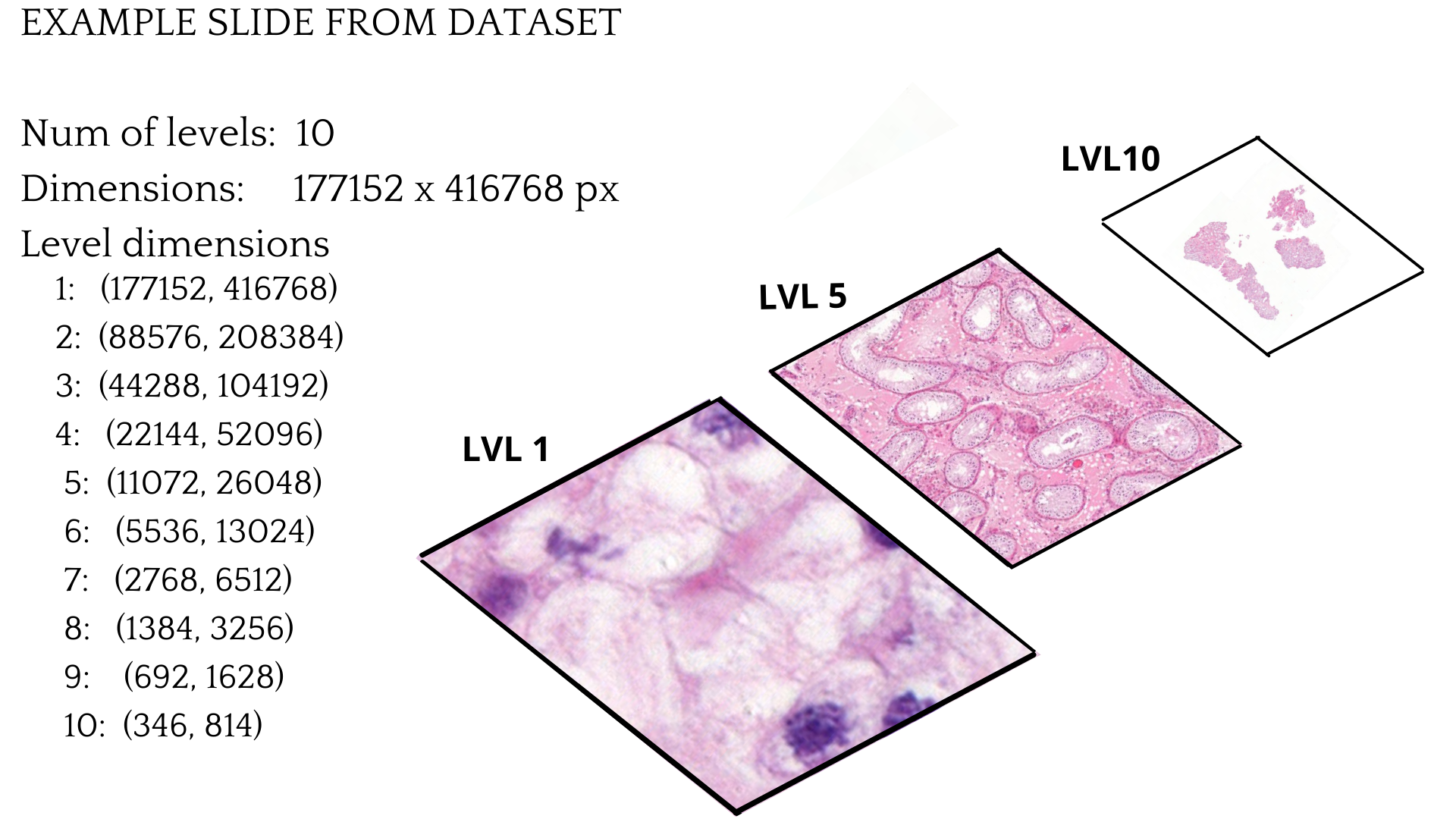
This is an example of a single training slide. The WSI image has ten different levels, with each layer becoming less detailed as the level grows. In this case, LVL 10 is the topmost layer and the one that has the smallest dimensions. The last layer can only be used for the image thumbnail. The LVL 1 is the lowest layer and has the highest dimensions. Also, this layer is the most precise. Another factor to consider is that most of the image is empty. Only a proportion of it is actual tissue, as can be seen from the LVL 10 image.
Training dataset
The training dataset consists of 4 WSI slides, and each slide has 200 annotations. These annotated cells are at different stages of the spermatozoid life cycle. Based on their proportions, one can diagnose infertility.
| Spermatozoid type | Annotated cell count |
|---|---|
| Spermatogonia | 181 |
| Primary spermatocyte | 180 |
| Spermatid | 180 |
| Sertoli | 179 |
| Spermatozoa | 80 |
Downscaling images
As the whole-slide images are too big to process, it was required to downscale the image into smaller tiles. For achieving smaller annotated images, the WSI was scanned with user-selected tile size. Then, annotations were collected for that tile, if any existed. The annotated cell center point was used to determine if the cell is on the tile or not. Finally, tiles and collected annotations were saved. I converted the original annotations into the COCO format for easier processing. COCO format could be used as an input for different models and frameworks and makes model/framework changing a lot easier if required.
FiftyOne dataset visualization
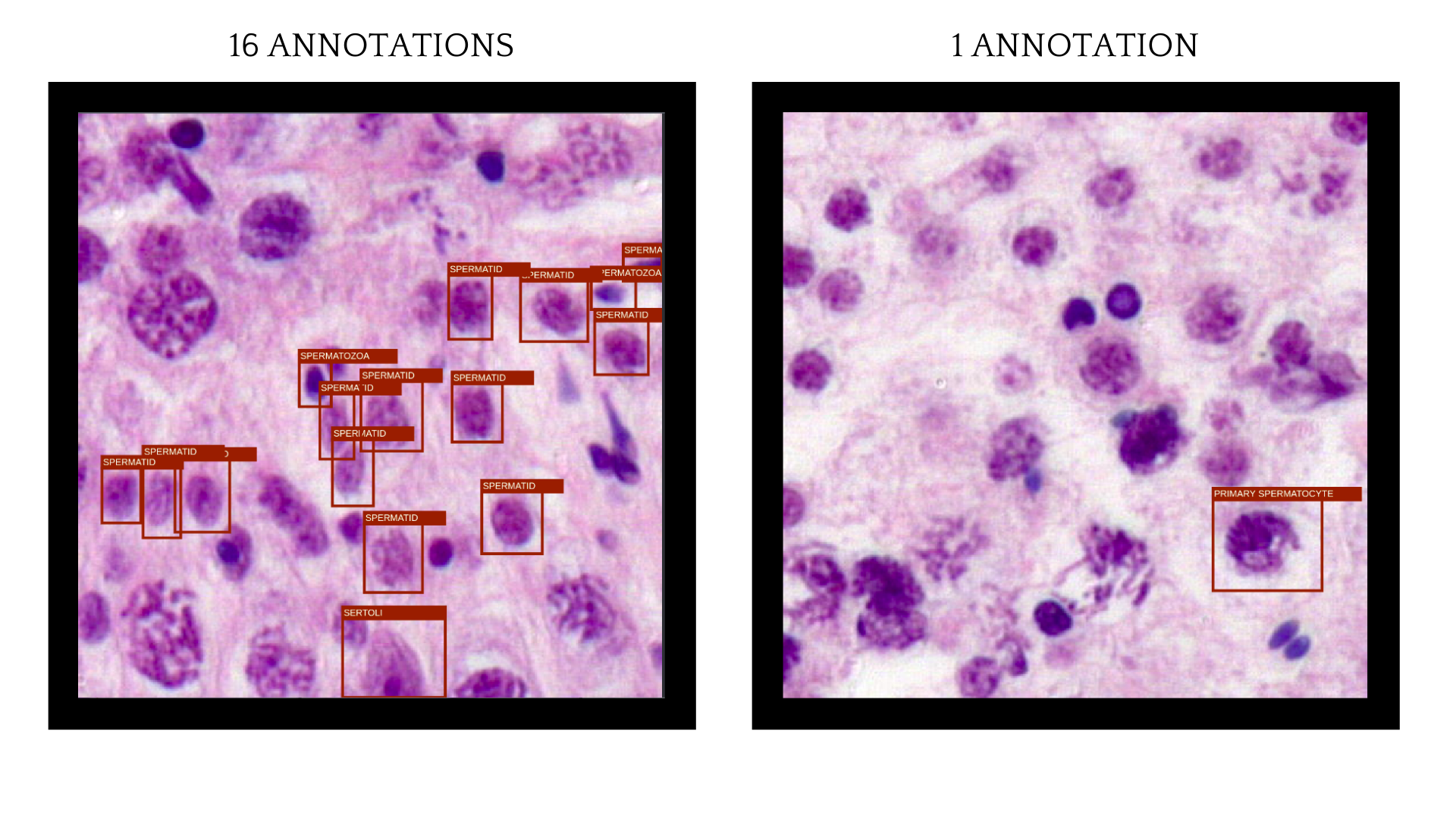
To get a better overview of the annotation correctness and insights of the data FiftyOne was used. FiftyOne is a great solution for dataset and model predictions visualization and finding mistakes in annotated images. Good overview of training dataset and prediction visualization help to understand insights of trained model much better. Some of the training images had many annotations, but there were images where only a singe annotated cell was visible.
Training detection model
After solving the downscaling problem and generating a dataset that can be trained upon it is time to select a machine learning framework and a model to train. There are multiple options here to go with, initially Center-Net, was the model in mind, but due to implementation difficulties Pytorch and Faster R-CNN architecture was used.
Custom data loader
To pass generated dataset to the Pytorch model a custom data loader needs to be implemented. Unfortunately there is a great tutorial how to implement the data loader for a custom COCO dataset. Also the Pytorch has a good boilerplate for detection training scripts found in their github repo. So combining these two great sources allowed to write the training script more easily.
Augmentations
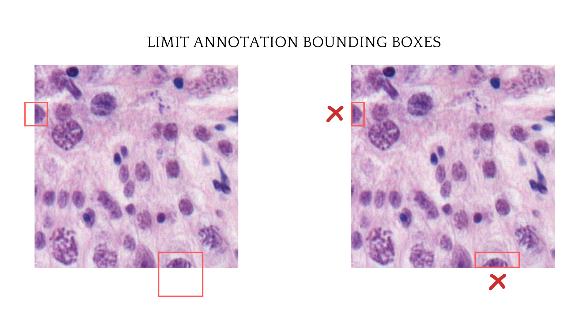
Detection task needs a little more work than classification task when it comes to image augmentation. The original bounding boxes on images also need to shift and follow the augmented image corresponding sections to match the cell after augmentation. Furthermore, as the annotation was considered on the image if the annotation center point was on the selected tile, then the bounding boxes shape also need to be limited by the image’s border.
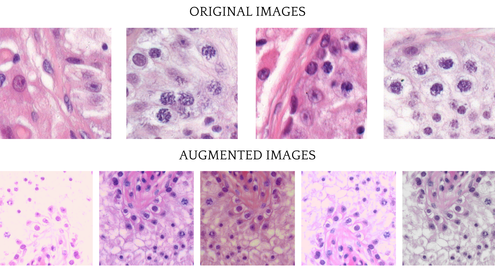
In order for the model to generalize and achieve better performance image augmentations were used in training process. Albumentations library was used in order to distort the original images. The training images transforms consisted of Flipping, RandomBrightnessContrast, HueSaturationValue augmentations and CLAHE or FancyPCA augmentations.
Training
Model was trained on the Tartu University HPC (High Performance Computing Center) using NVIDIA Tesla V100 GPU.
Using images from different levels
After implementing the first model with only level 1 (the layer with largest dimensions) images, the model might improve by seeing cells from different heights as humans do when annotating different cell types. The level 1 image might provide more essential details on how the exact cell looks and how to distinguish it from other cells. However, the higher-level images might provide an overview regarding cell positioning, detection, etc.
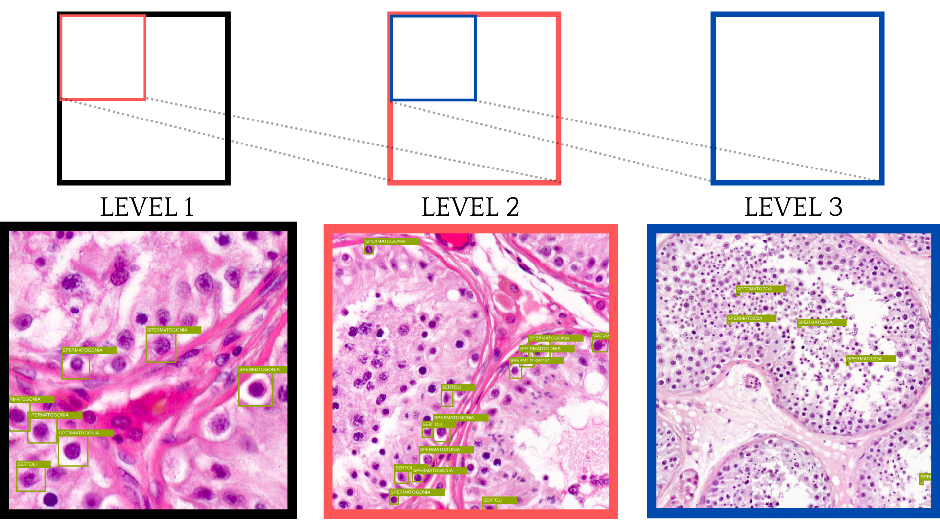
Taking images from different layers also meant that the bounding boxes for layer one needed to be scaled accordingly. As each level was scaled to cover twice the dimension of the previous one, then using images above level 3 seemed to be ineffective as the annotations got smaller and smaller.
Validation
Eliminating predictions
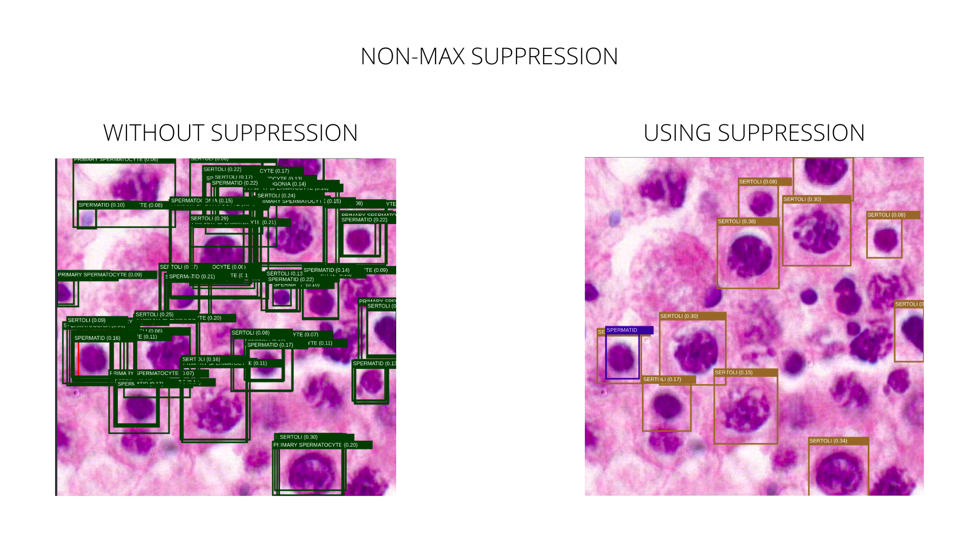
Non-Max Suppression is a technique to filter the predictions of object detections. The idea of the Non-Max Suppression is to keep the highest-scoring bounding box for a single detection. The IOU (intersection over union) of two bounding boxes is calculated to determine if the boxes overlap and the lowest scoring boxes are dropped. This method can reduce the prediction noise quite a lot, as seen in the following image.
Current issue with annotations
The model doesn’t perform too well because of the current annotation logic. The slides are not fully annotated, and only some cells on the sampled images have labels. While collecting tiles, some cells on an image have annotation, and some don’t. Two visually identical cells can be side by side, but only one of them, a labeled one, is considered a detection, and an unlabeled cell is considered noise. This behavior allows the model to find cells but not to distinguish between different types.
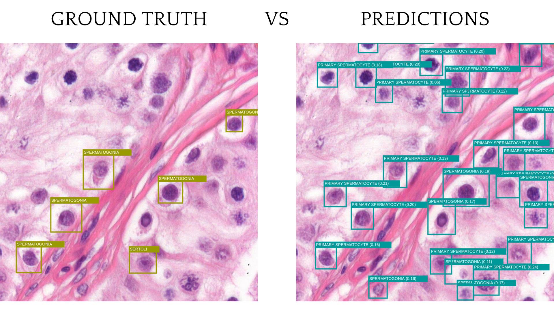
The solution might be to create a slide or a region that has all of the correct cells annotated and use this slide for training.
Conclusion
There is a lot of work before training the neural network model. Data comes in different formats, and the preprocessing takes most of the time. Also, the job isn’t finished when you have reached the model training phase. So there is always room for improvement. Otherwise, lots of new knowledge with WSI, Pytorch, Python, FastPages, using HPC Cluster, etc.
Source Code available in:
GitHub
